Open Science

• Introduction to some of the best tools for doing Reproducible Research
  • R & RStudio (swirl modules 1 and 2)
  • (R)Markdown (examples)
  • Git & GitHub (Sign up on GitHub and email your username)
  • Zenodo, OSF (Sign up on Zenodo using your GitHub account)

install.packages("swirl") # Install the swirl package
library("swirl") # Load the swirl package in the R environment
swirl() # Start swirl

You are prompted to install a course, and a list of 5 options is offered. Select option '5. Don't install anything for me. I'll do it myself'. A GitHub page will open and the swirl session will close. We want to install the R_Programming_E course. Back to RStudio, type in the console

install_course_github("swirldev", "R_Programming_E")
swirl() # Start again swirl

You should now see listed the course '1: R Programming E'

1: Basic Building Blocks

• create variables
• numeric vectors
• c() function
• ?, help() functions
• vectorization
• arithmetic operations
• sqrt(), abs() functions
• auto-complation (Tab) and command history (Up arrow)

Would you like to inform someone about your successful completion of this lesson via email? Select '1. Yes', type in your full name and my email address domenico.giusti@uni-tuebingen.de. Your email client should open. Send that email.

2: Workspace and Files

• getwd(), setwd() functions
• ls(), list.files() functions
• args() function
• dir.create(), file.create() functions
• file.exists(), file.info(), file.rename(), file.copy(), file.remove(), file.path() functions

Your operating system and RStudio provide simpler graphic tools for these sorts of tasks, but having the ability to manipulate files programatically is useful in reproducible research. Also useful when working with dozens, thousands or milions of files.

If you have to repeat the same tasks more than [individual threshold], code them once!

Complete swirl modules '3: Sequences of Numbers' and '4: Vectors' and submit your successful completion via email (domenico.giusti@uni-tuebingen.de)

swirl modules won't count towards your final grade but are highly recommended to follow.

Managing your projects in a reproducible fashion doesn't just make your science reproducible, it makes your life easier. @vsbuffalo

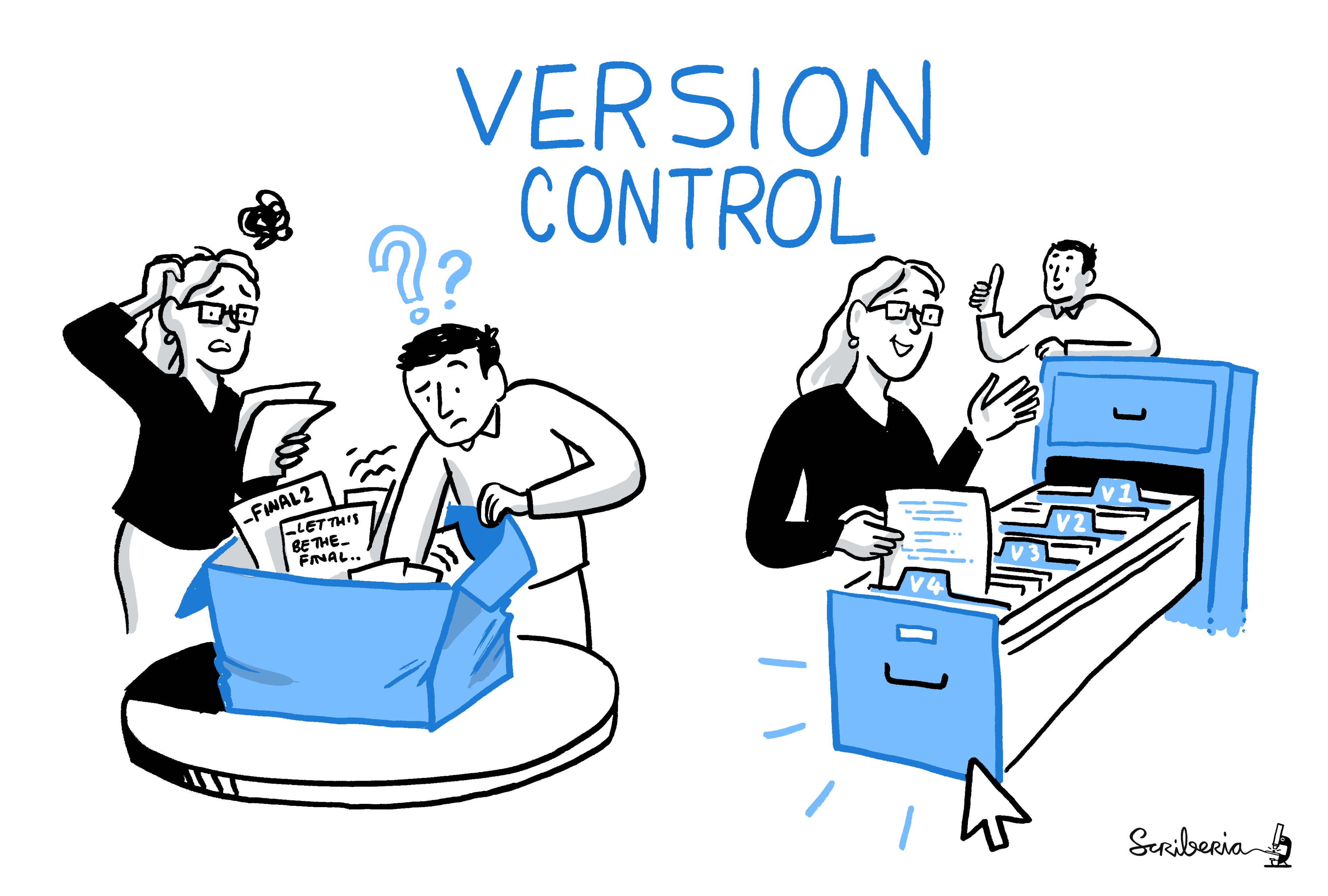
This image (and the previous one) was created by Scriberia for The Turing Way community and is used under a CC-BY licence

We’re going to create a new project in RStudio:

1. Click the “File” menu button, then “New Project”.
2. Click “New Directory”.
3. Click “New Project”.
4. Type in the name of the directory to store your project, e.g. “test_rr”.
5. (Sip Git for now...)
6. Click the “Create Project” button.

An .Rproj file is created in your project directory. All your data, plots and scripts will now be relative to the project directory.

Put each project in its own directory, which is named after the project.

PhD comics

• It keeps raw (original) and processed (modified) data separated -> Ensure the integrity of your data
  • Treat raw data as read only! Working with raw data interactively (e.g., in Excel) means that you will overwrite the original format, and with no track changes you won't know how it has been modified.
  • Store processed data in a separate file. Significant preprocessing is often needed to get your raw data into a tidy format for analysis.
• It keeps organized in different folders files with different extensions -> Makes easier to find things
• It keeps your code and output in different folders -> Treat generated output as disposable
  • Many analyses are exploratory and don’t end up being used in the final project, and some of the analyses get shared between projects.

• It keeps separate function definition and application
  • When your project is in its early stages, the initial .R script file usually contains many lines of directly executed code. As it matures, reusable chunks of code are saved as R functions. It’s a good idea to separate these functions into two separate folders; one to store useful functions that you’ll reuse across analyses and projects, and one to store the analysis scripts.
• It makes it simpler to share your project with someone else, to upload data/code with your manuscript submission, to pick the project back up after a break.

For this exercise we are going to use the archdata. "The archdata package provides several types of data that are typically used in archaeological research. It provides all of the data sets used in Quantitative Methods in Archaeology Using R" by David L Carlson."

You can get the whole collection of datasets by installing the package 'archdata'

install.packages("archdata")

The collection is released under the GNU GENERAL PUBLIC LICENSE GPL3. Read the package reference manual.

Create a new .Rmd file in your RStudio 'test_rr' project.

# load the Acheulean dataset
install.packages("archdata") # install the package
library(archdata) # load the package
data(package="archdata") # show the data sets in package ‘archdata’
data("Acheulean") # load the Acheulean data set in the R Environment
?Acheulean

# create a /data directory
getwd() # get working directory
list.files() # list files in the wd
dir.create("data") # create a /data directory

# download the data from Dropbox
url <- "https://www.dropbox.com/s/zpf2062jrdbhj2s/Acheulean.csv?raw=1"
# NOTE: add a raw=1 URL parameter or you will get a HTML preview page,
# not the file content itself
destfile <- "data/Acheulean.csv" # specify destination where file should be saved
download.file(url, destfile) # download the CSV file

# read the CSV file
Acheulean <- read.csv(file = "data/Acheulean.csv",
                      header = TRUE, sep = ",", dec = ".", row.names = 1)
# There are functions to read as well Excel files.

First look at the dataset

View(Acheulean)
str(Acheulean) # data object stucture
summary(Acheulean) # summary

"80% of data analysis is spent on the cleaning and preparing data. And it’s not just a first step, but it must be repeated many times over the course of analysis as new problems come to light or new data is collected." Tidy Data

Data structure:

• Every column is a variable and contains one "type" of data
  • Logical (TRUE, FALSE)
  • Numeric (12.3, 5, 999.99)
  • Integer (1, 2, 3, 4)
  • Character (a, good, 'TRUE', '12.3')
  • Factor (male, female)
• Every row is an observation.
• Every cell is a single value.

"Real datasets can, and often do, violate the three precepts of tidy data in almost every way imaginable. While occasionally you do get a dataset that you can start analysing immediately, this is the exception, not the rule." Tidy Data

• Column headers are values, not variable names.
• Multiple variables are stored in one column.
• Variables are stored in both rows and columns.
• Multiple types of observational units are stored in the same table.
• A single observational unit is stored in multiple tables.

data(Acheulean)
# Compute percentages for each assemblage
Acheulean.pct <- prop.table(as.matrix(Acheulean[,3:14]), 1)*100
round(Acheulean.pct, 2)
plot(OST~HA, Acheulean.pct)
boxplot(Acheulean.pct)

• Save your .Rmd file
• Save your RStudio project (.Rproj)
• Save workspace image to ~/nextCloud/Teaching/Open science/test_rr/.RData?
  • SAVE!
  • An hidden .RData file is saved in the project directory
• An hidden .Rhisory is also saved in the project directory

• CRAN Task View: Archaeological Science